SVD

Introduction

Posted on September , 2023 in JayanthBlog

I don't know how to start, but I'll start. Many of us had the idea that math was boring, but it actually isn't. In the beginning of my math journey, I wondered why we use math in all fields like science, physics, and economics. After exploring linear algebra , quadratic programming and optimization problem , I realized that I had missed a lot of things, and my perspective on math completely changed. Coming to today's topic, SVD, also known as Singular Value Decomposition (SVD), is a mathematical technique used for factorizing a matrix into three simpler matrices. Actually, it is singular, and we have to express the matrix as a product of three values, but it's okay; we can express it like this. First, let's discuss some of the math concepts and also express them in the form of SVD.

Before we dive into the topic, do you have a basic understanding of linear transformations? Let's forget about the calculations for now and focus solely on the geometrical intuition. Imagine you have a piece of paper with a drawing on it. A linear transformation is akin to taking that piece of paper and stretching it, squashing it, or flipping it around, but without tearing or folding it. As a result, the drawing on the paper changes its shape, but it remains fundamentally the same drawing. This is what we refer to as a linear transformation, like giving the drawing a magical makeover

 consider a matrix  A =[ 3 , 1 ]
                       [ 4 , 5 ]
    (x, y ) in the form of (3x+y , 4x+5y)
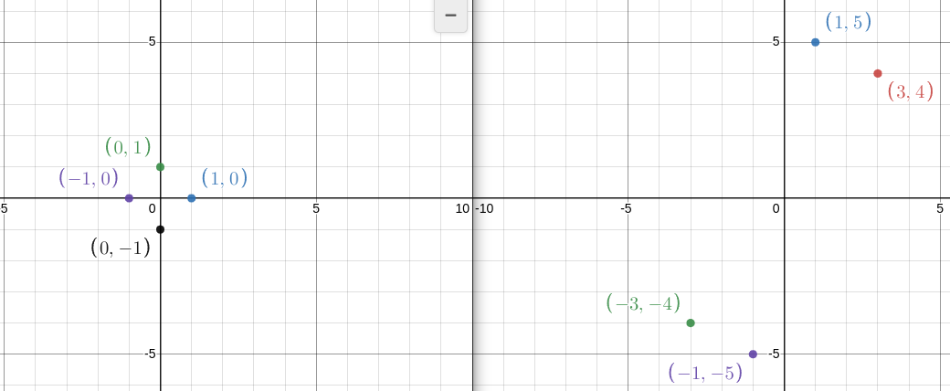
    (1,0) => (3,4)
    (0,1) => (1,5)
    (-1,0) =>(-3,-4)
    (0,-1) => (-1 ,-5)
    applied a magical process and obtained new coordinates (x, y) transformed into the form (3x + y, 4x + 5y).
    Now, let's substitute the following points: (1, 0), (0, 1), (-1, 0), and (0, -1), 
    and then plot them on a graph to observe the transformation.
        

Conclusion: Even though you place a small point at (1, 0), it transforms the circle into an ellipse. This is the beauty of linear algebra.

SVD factorizes A into three matrices: U: An m x m orthogonal matrix (U^T * U = I), where U^T represents the transpose of U. Σ (Sigma): An m x n diagonal matrix with non-negative real numbers on the diagonal. These diagonal values are called singular values and are arranged in descending order. V^T (the transpose of V): An n x n orthogonal matrix (V^T * V = I) .
A = U * Σ * V^T
Before Singular Value Decomposition (SVD), there is another concept used to transform square matrices called eigen-decomposition. However, eigen-decomposition has some limitations, which is why SVD is used. SVD can be applied to any m×n matrix. In SVD, a matrix is transformed into three matrices: U, Σ, and V^T. To explain these terms from last to first, V^T is an orthogonal matrix that you can think of as responsible for rotation, Σ is for scaling, and U is also involved in rotation. That's it; this is a simple explanation of SVD. Don't worry about the calculation part; we are not mathematicians; we are programmers. So, I'll take a simple matrix and demonstrate how to transform it into the three SVD matrices

 consider a matrix  A =[ -4 , -7 ]
                       [ 1 , 4 ]
    A*A^T = [65 , -32]
            [-32 , 17]
    it is simply matrix and it transpose multiplication 
    and calculate characterstic equation we get  λ^2 -82λ + 81 = 0 
    eigen values λ = 1, 81 
    eigen vector λ1 (1) = [0.5 , 1]2X1 
    eigen vector λ2 (81) = [-2 , 1]2X1
    normalize the eigen vector by magnitute we get 
    eigen vector λ1 (1) = [0.447 , 0.894]2X1 
    eigen vector λ2 (81) = [-0.894 , 0.447]2X1
    U = [0.447 , 0.894]
        [-0.894 , 0.447] 2x2
    Σ =  [9 , 0]
         [0 , 1] # square of eigen vector 
    V^T = According to the Grahm-Schmidt orthogonalization process we get 
        = [0.447 , -0.895]
          [0.894 , 0.447]
    I think your mind is now full of calculations, so I generally don't prefer this method.
    Actually, programmers are lazy, so we like to reuse code efficiently.
    Another fellow programmer has developed some functions..
 

Here a code sample in Python

1. import numpy as np
2. A = [[-4 , -7] , [1, 4]]
3. U, S, VT = np.linalg.svd(A) #function for svd in python
4. print(U)
5. print(S)
6. print(VT)

its matter of 2 lines  

I think I've covered the mathematical aspect of SVD. Now, let's move on to programming and explore image compression. Let's get started.

Here a code for compression of images in python

Original Image

1. #import dependencies
2. import numpy as np
3. from numpy.linalg import svd
4. import matplotlib.pyplot as plt
5. from matplotlib.pyplot import imshow

In the previous example, I used NumPy for mathematical operations and Matplotlib to display images. Now, I am going to define a function that will take a matrix as input...

1. vmin = 0 #for white
2. vmax = 1 #for black
3. image_bias = 1 # sometimes 1
4. def plot_svd(A):
5. n = len(A)
6. imshow(image_bias-A, cmap='gray', vmin=vmin, vmax=vmax)
7. plt.show()
8. U, S, V = svd(A)

1. imgs = []
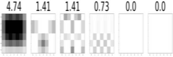
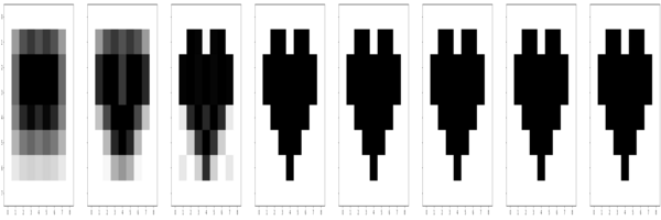
2. for i in range(n):
3. imgs.append(S[i]*np.outer(U[:,i],V[i]))
5. combined_imgs = []
6. for i in range(n):
7. img = sum(imgs[:i+1])
8. combined_imgs.append(img)
9. fig, axes = plt.subplots(figsize = (n*n,n), nrows = 1, ncols = n, sharex=True, sharey=True)

Images of all eigenvalue of an images

1. for num, ax in zip(range(n), axes):
2. ax.imshow(image_bias-imgs[num], cmap='gray', vmin=vmin, vmax=vmax)
3. ax.set_title(np.round(S[num],2), fontsize=80)
4. plt.show()
6. fig, axes = plt.subplots(figsize = (n*n,n), nrows = 1, ncols = n, sharex=True, sharey=True)
7. for num, ax in zip(range(n), axes):
8. ax.imshow(image_bias-combined_imgs[num], cmap='gray', vmin=vmin, vmax=vmax)
9. plt.show()

Compression of an image at each stage by adding all the eigenvectors of the image can result in a clearer image.